Time Complexity tells us about how long an algorithm takes to execute, relative to its input size. It is a quick way to understand the relative performance of an algorithm.
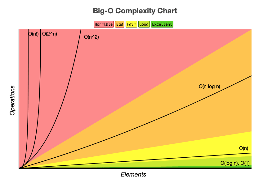
The graph below gives us a quick idea of the time complexities we are going to cover in this article:

Table of contents:
- What is Time Complexity?
- What is BigO?
- O(1) Constant Time
- O(logn) Logarithmic Time
- O(n) Linear Time
- O(n^2) Quadratic Time
- O(2^n) Exponential Time
In this article, I am going to talk about Time Complexity, what is BigO and how BigO helps us to improve our algorithms.
So let's start with what is Time Complexity.
1. What is Time Complexity
Time Complexity is how much time an algorithm takes to execute. But we are not going to calculate the exact time for an algorithm execution. Instead of that, we are going to calculate how much the input size affects our algorithm's execution time.
2. What is BigO?
"BigO notation is a mathematical notation that describes the limiting behavior of a function when the argument tends towards a particular value or infinity." -Wikipedia
For example, we have O(1) which stands for Constant Time, which means that our algorithm's execution time doesn't change with input size.
Now that we've seen what Time Complexity and BigO mean, let's see what kind of BigO notations we have and what they mean.
3. O(1) Constant Time
An algorithm whose time complexity doesn't change with input size. It is that simple!
For example, getting the first element from a list. The input size doesn't affect this algorithm, because the first element is always first no matter how much input size is.
def get_first(data):
    return data[0]

data = [1, 2, 3, 4]
get_first(data)
4. O(logn) Logarithmic Time
Here is a quick reference for "What is a Logarithm": https://byjus.com/maths/logarithms/. A logarithmic algorithm splits a list or other data structure into smaller pieces every time it runs.
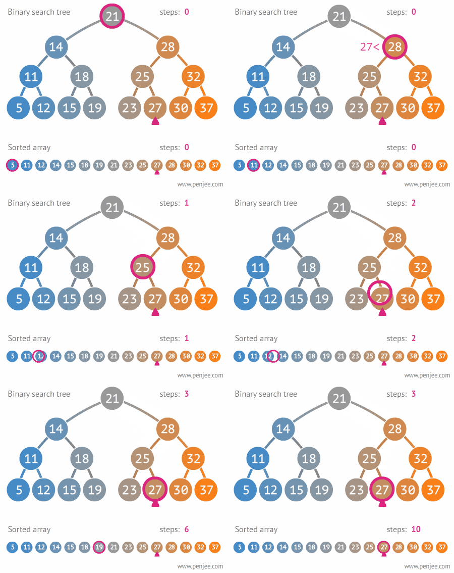
The best example of an algorithm that has an O(logn) Time Complexity is "Binary Search". Binary search must be performed on a sorted list.
Let's look at the implementation.
# Iterative Binary Search Function
# It returns the index of x in the given list if present,
# else returns -1
def binary_search(lst, x):
    low = 0
    high = len(lst) - 1
    mid = 0

    while low <= high:

        mid = (high + low) // 2

        # If x is greater, ignore the left half
        if lst[mid] < x:
            low = mid + 1

            # If x is smaller, ignore the right half
            elif lst[mid] > x:
            high = mid - 1

            # means x is present in mid
            else:
                return mid

        # If we reach here, then the element was not present
        return -1


# Test list
lst = [ 2, 3, 4, 10, 40 ]
x = 10

# Function call
result = binary_search(lst, x)

if result != -1:
    print("Element is present at index", str(result))
else:
    print("Element is not present in list")
Let me explain what this algorithm is all about in English.
- Go to the middle of the list.
- Check to see if that element is what we are searching for.
- If it's not then check if the element that we are looking for is greater than the middle element.
- If it is, then ignore the right side of this list after now, otherwise, ignore the left side of this list after now.
- With the list we are left with, repeat steps 1 to 4.

Compared with the Linear (Sequential) Search
5. O(n) Linear Time
In linear time algorithms every single element in the input is visited once. As the input size grows our algorithm's run time grows exactly with the size of the input.
Linear search is an example of an algorithm of linear complexity.
Here is the implementation:
#Define the linear search function
def search(lst, x):

    for i in range(len(lst)):

        if lst[i] == x:
            return i

    return -1

#Let's give it a try
lst = ["a","b","c","find me","d"]

print(search(lst, "find me"))

>>3
6. O(n^2) Polynomial Time
An algorithm that may visit every element once is a linear algorithm, O(n). Usually this is accomplished with a loop that iterates over every element of a list.
But what if you have nested loops, like in this example?
lst = [1, 3, 5]
for x in lst:
    for y in lst:
        pass
If this was an O(n) algorithm, we would perform a total of 3 iterations, since the list has 3 elements. But with nested loops, we end up performing 9 iterations. This is why the time complexity is polynomial, O(n^2), because 3^2 = 9.
Bubble Sort is a very good example of this:
def bubbleSort(lst):
    n = len(lst)

    # Traverse through all list elements
    for i in range(n):

        # Last i elements are already in place
        for j in range(0, n-i-1):

            # traverse the list from 0 to n-i-1
            # Swap if the element found is greater
            # than the next element
            if lst[j] > lst[j+1] :
                lst[j], lst[j+1] = lst[j+1], lst[j]

# Driver code to test above
lst = [64, 34, 25, 12, 22, 11, 90]

bubbleSort(lst)
The bubble sort algorithm takes the first number and swaps it with the adjacent number if they are in the wrong order. It does this for each number until all numbers are in the right order - and thus sorted.

7. O(2^n) Exponential Time
This is absolutely the worst one because it is the slowest!
Exponential time is 2^n, so the runtime grows exponentially with the size of the input.
Say we have a password consisting only of numbers (so that’s 10 numbers, 0 through to 9). we want to crack a password that has a length of n, so to brute force through every combination we’ll have 10^n.
As an example, let's say we want to create a password that has 15 characters in length! Quantity of the all combinations would be equal to 10^15 = 1.000.000.000.000.000!
An example for an exponential time algorithm is the recursive calculation of Fibonacci numbers:
def fibonacci(n):
    if n <= 1:
        return n
    return fibonacci(n-1) + fibonacci(n-2)
So, it is obvious that we don't want to use an algorithm that has an O(2^n) right? What can we do to deal with this problem? Let me explain it by an example.
Let’s say we have to calculate 10^4. We need to do this:
10 * 10 * 10 * 10 = 10^2 * 10^2
As you can see we have to calculate 10^2 two times. Why not calculate it one time and use the same result again? This approach is called Dynamic Programming. Here is an article to learn more about it!
Do not forget that knowing time complexities allows us to build better algorithms. We can use our knowledge to improve the algorithms because we know what causes a worse or better time complexity.
If you want to visualize the algorithms that we covered and more you can visit visualgo!
Here is a graph where you can see the time complexities that we covered.

Thanks for reading and I hope it helped you!
If you want to see my other articles and see posts about Python and Backend Development, check out my Twitter and Blog.
Extra Reading:
- https://skerritt.blog/all-you-need-to-know-about-big-o-notation-python-examples/
- https://www.geeksforgeeks.org/python-program-for-linear-search/
- https://towardsdatascience.com/understanding-time-complexity-with-python-examples-2bda6e8158a7
- https://www.geeksforgeeks.org/python-program-for-binary-search/

